Statistics: Grouped Data, Averages, Spread, Correlation and Regression

How WAEC marks statistics

WAEC gives marks for each stage: B1 for a correct table (x, f, fx, cf …), M1 for the correct formula and substitution, and A1 for an accurate answer. On graphs, a sensible scale, labelled axes and accurate plotting each earn marks. Table first, formula next, substitute, then answer with units.

Frequency tables for grouped data

Our main data set: the marks of 50 SS3 students in a Further Maths test.

• 10–19: f = 3 (cf 3)
• 20–29: f = 6 (cf 9)
• 30–39: f = 9 (cf 18)
• 40–49: f = 13 (cf 31)
• 50–59: f = 10 (cf 41)
• 60–69: f = 6 (cf 47)
• 70–79: f = 3 (cf 50)

Key words for the class 10–19:

• Class boundaries: 9.5 – 19.5 (lower limit − 0.5, upper limit + 0.5)
• Class width: 19.5 − 9.5 = 10
• Class mark (midpoint): (10 + 19) ÷ 2 = 14.5
• Cumulative frequency (cf): the running total of frequencies, ending at N = 50

Histogram and frequency polygon

• Plot class boundaries on the x-axis, so the bars touch.
• Bar height = frequency (when the widths are equal).
• Frequency polygon: join the midpoints of the bar tops, and close it at both ends.

Unequal class widths: the bar height must be the frequency density = frequency ÷ class width, so that the area of each bar shows the frequency.

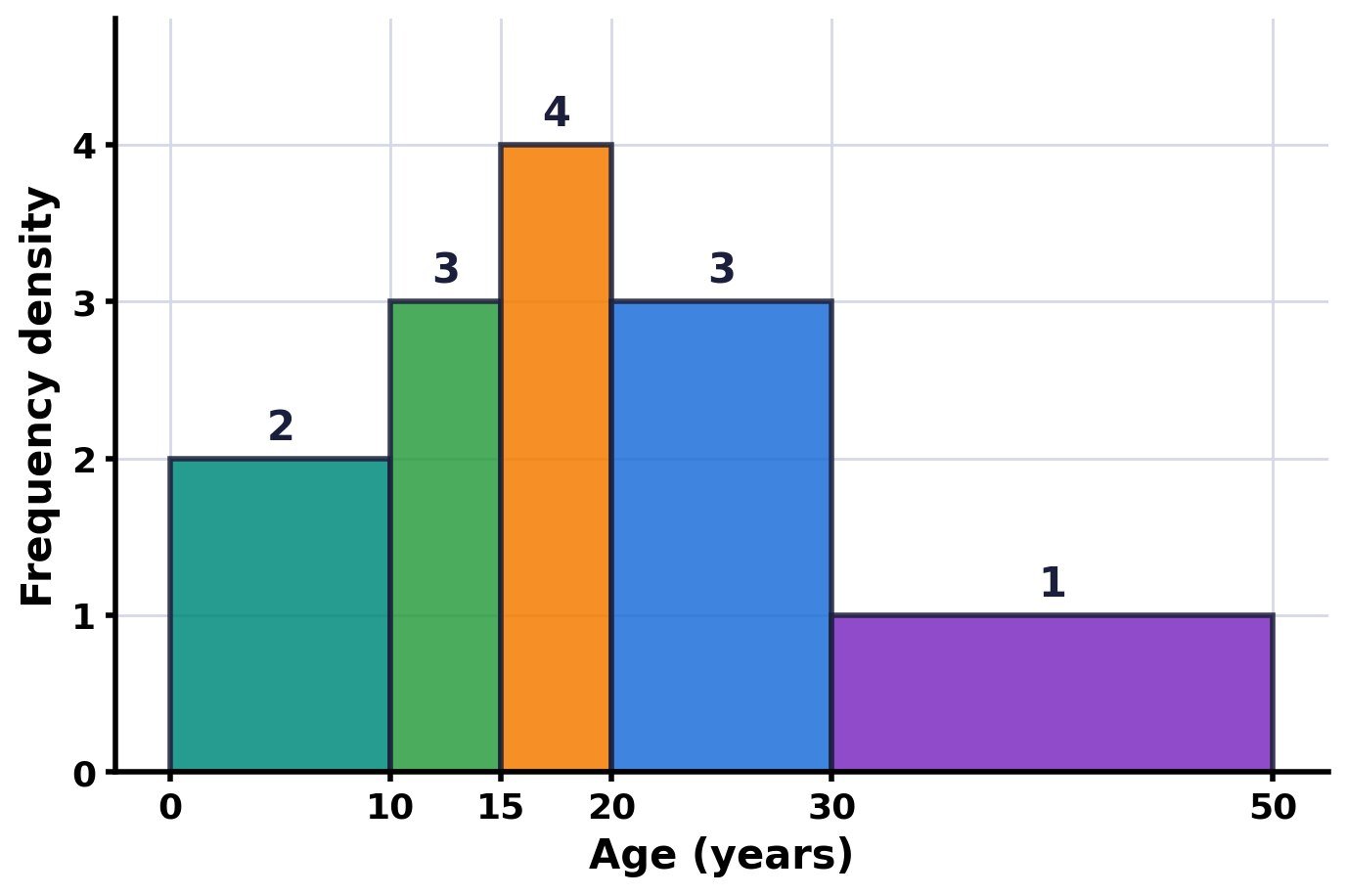
The ogive (cumulative frequency curve)

• Plot (upper class boundary, cf), starting at (9.5, 0), and join with a smooth S-shaped curve.
• Read across at N/4 (lower quartile Q₁), N/2 (median) and 3N/4 (upper quartile Q₃).
• Interquartile range IQR = Q₃ − Q₁; semi-interquartile range = ½(Q₃ − Q₁).

The mean by assumed mean and coding

Choose an assumed mean A (a midpoint near the middle) and the class width c, then code: u = (x − A)/c.

x̄ = A + c × (Σfu ÷ Σf)

The median and quartiles by formula

Median = L₁ + [(N/2 − F) ÷ f] × c

where L₁ = lower boundary of the median class, F = cumulative frequency before that class, f = its frequency and c = class width.

The same formula gives the quartiles, using N/4 and 3N/4 instead of N/2.

The mode

Mode = L₁ + [Δ₁ ÷ (Δ₁ + Δ₂)] × c

where Δ₁ = (modal frequency − frequency before) and Δ₂ = (modal frequency − frequency after).

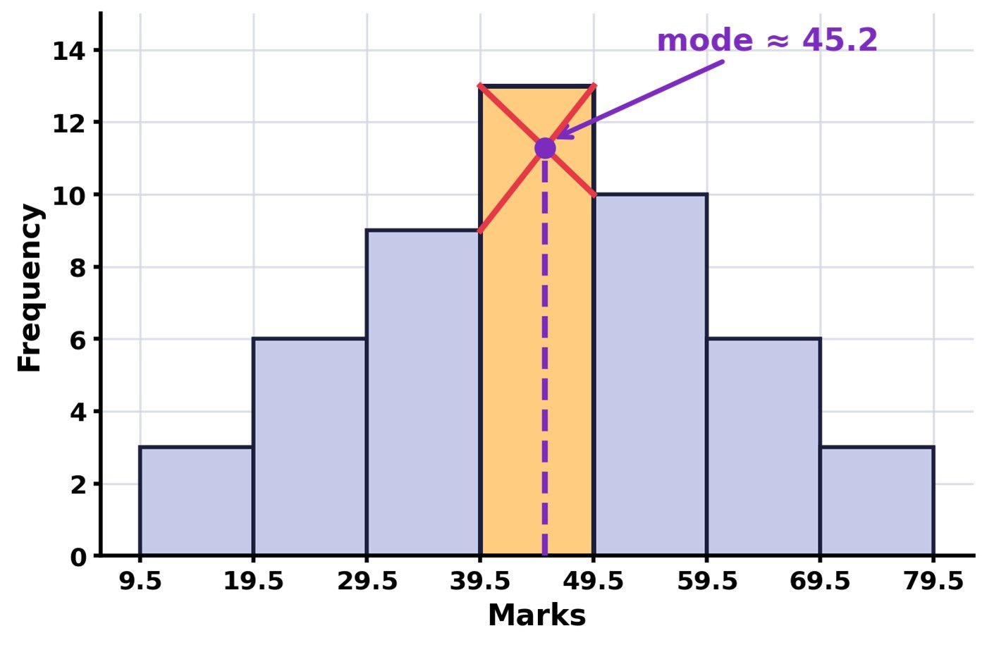
Comparing the averages: mean 44.7, median 44.9, mode 45.2 are almost equal, so the marks are spread fairly symmetrically. A mean much higher than the median suggests a right (positive) skew; much lower, a left (negative) skew.

Measures of spread

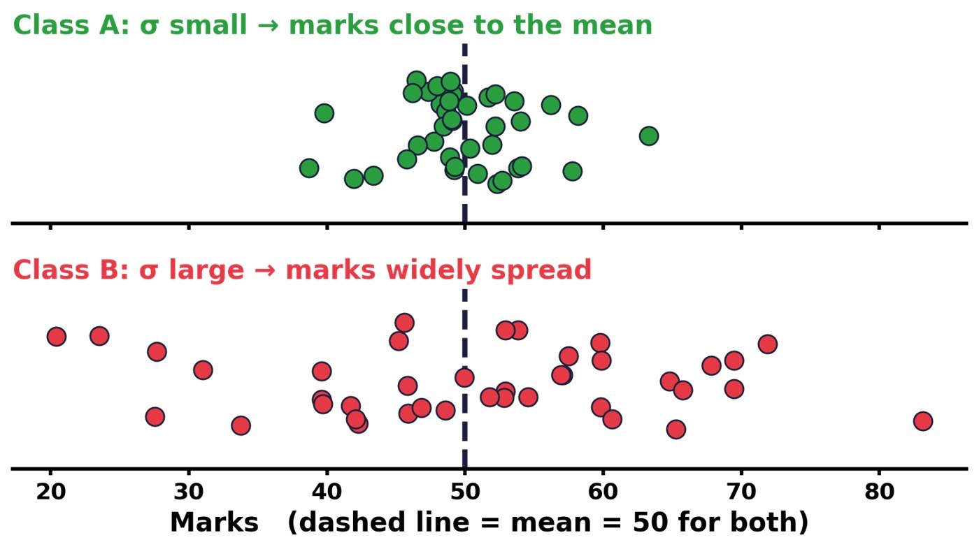
Two classes can have the same mean but very different spreads. Measures of spread:

• Range = highest − lowest
• IQR = Q₃ − Q₁ (not affected by extreme values)
• Mean deviation = Σf|x − x̄| ÷ Σf
• Variance σ² = Σf(x − x̄)² ÷ Σf, and standard deviation σ = √variance

Standard deviation of grouped data by coding:

σ = c × √[Σfu²/Σf − (Σfu/Σf)²]

What happens when every value is changed?

• Add k to every value: the mean becomes x̄ + k; the standard deviation is unchanged.
• Multiply every value by a: the mean becomes ax̄; the SD becomes |a|σ; the variance becomes a²σ².
• Both (ax + k): the mean becomes ax̄ + k; the SD becomes |a|σ.

Correlation

A scatter diagram shows whether two variables move together: positive (e.g. study hours and scores), negative (e.g. speed and journey time) or none (e.g. height and exam score).

Spearman's rank correlation coefficient:

ρ = 1 − 6Σd² ÷ n(n² − 1)

where d is the difference between the two ranks of each item and n is the number of pairs. −1 ≤ ρ ≤ 1: close to +1 is strong positive, close to −1 is strong negative, near 0 is little or no correlation.

The least-squares regression line

The line of best fit y = a + bx has:

b = (nΣxy − ΣxΣy) ÷ (nΣx² − (Σx)²) and a = ȳ − bx̄

The line always passes through the mean point (x̄, ȳ). Only predict inside the range of the data (interpolation). Predicting outside it (extrapolation) is unreliable.

Which tool do I need?

• Where is the centre? Mean (coding), median and quartiles, mode
• How spread out? Range, IQR, mean deviation, variance and SD
• What shape? Histogram (density if widths are unequal), frequency polygon, ogive
• Two variables? Scatter diagram, Spearman's ρ, regression line

Practice

1. The mean of 3, 5, x, 9 and 11 is 7. Find x.
2. A set of data has SD 4. Each value is multiplied by 3 and then 2 is added. Find the new SD.
3. For n = 5 pairs, Σd² = 4. Find Spearman's ρ.
4. The regression line y = 3 + 2x passes through (x̄, ȳ). If x̄ = 4, find ȳ.
5. Find the mean deviation and standard deviation of 3, 5, 6, 8, 13.
6. The masses of 60 students are: 40–44 (4), 45–49 (9), 50–54 (15), 55–59 (18), 60–64 (10), 65–69 (4). Find the mean using A = 57 and c = 5, and the median.

Answers: 1. x = 7 · 2. 12 · 3. ρ = 1 − 24/120 = 0.8 · 4. ȳ = 11 · 5. x̄ = 7; MD = 14 ÷ 5 = 2.8; σ² = 58 ÷ 5 = 11.6, so σ ≈ 3.41 · 6. Σfu = −27, so x̄ = 57 + 5(−27/60) = 54.75 kg; median = 54.5 + [(30 − 28) ÷ 18] × 5 ≈ 55.1 kg

Previous topic: Work, Energy and Power.